Compression and Intelligence

Part One: Compression

Pretraining

Pretrained large language models are famously next-token predictors. The procedure of pretraining consists of randomly initializing a (typically Transformer) model $\theta$, taking a sequence of data $X = (x_1, x_2, \dots, x_T)$, autoregressively predicting the probabilities of each symbol: $p_\theta\left(x_t \mid x_{\lt t}\right)$, computing a loss $\ell$ of how well the model predicted the true sequence $X$, and backpropagating $\ell$ to adjust the model’s weights to make $X$ more likely, with the hope that the absorbed regularities will help predict future sequences.

What does this have to do with compression? Well, we can convert the probabilities to surprisal: $-\log_2 p_\theta\left(x_t \mid x_{\lt t}\right)$. The unit of surprisal is the bit: surprisal quantifies the minimum number of bits needed to losslessly encode $x_t$ in such a way that it can be decoded by anyone with $p_\theta$. The total number of bits $L$ needed to encode $X$ is therefore:

The better $\theta$ is at predicting $X$, the smaller $L_\theta(X)$, the fewer bits it needs to encode it. $L_\theta(X)$ is the theoretical lower bound of bits needed to encode the data (conditioned on $\theta$), but in practice entropy coding algorithms like arithmetic coding get extremely close to it (within a couple of bits for long sequences of data).

All predictive models, such as pretrained language models, can be leveraged to losslessly compress sequences of data in this way, but the relation between pretraining and compression is even more direct. The loss function $\ell$ used to pretrain language models is cross-entropy¹, the average surprisal:

The pretraining of large language models explicitly optimizes their ability to encode sequences of data in as few bits as possible.

Offline Compression

To illustrate how effectively pretrained language models can be used for compression, following the general approach from Delétang et al. (2023) we will use the predictions of pretrained models from the Qwen3 series (Yang et al. 2025), along with the arithmetic coding implementation from constriction, to encode a variety of datasets, and compare their compression efficiencies with that of the traditional compression algorithms gzip and zstd.²

The datasets we’ll look at are the following. The first two were selected because they were published a year after the weights of the Qwen3 models were released, helping to ensure they are not already in the weights, while the last was selected due to its unique density of semantic meaning.

• Infini-News 2026: A 1 MB subset of text from English 2026 news articles taken from the Infini-News dataset (Lazzaroni et al. 2026)
• Magnifica humanitas: The 239 KB text of Pope Leo XIV’s first encyclical (concerning artificial intelligence) published in May 2026
• Finnegans Wake³: The 1.4 MB text of James Joyce’s final novel, which was written in an idiosyncratic language “alleged to achieve a compression of semantic content” (Shannon, 1948)

To compare the compressed file sizes across the models and traditional compression algorithms, we will express their efficiencies in terms of bits-per-byte (bpb), which is simply the length of the encoded bitstream $L_\theta(X)$ divided by the total number of bytes in the raw UTF-8 text (so uncompressed text sits at 8.0 bpb), as the metric expresses compression efficiency in a way that is agnostic to the compressor’s input encodings (tokens vs. bytes) and is normalized across the size of the datasets.

Even the smallest model compresses each dataset to a significantly smaller size than both gzip and zstd, and as the models grow in size — as they become stronger predictors — they compress the contents into fewer and fewer bits.

However, in order to decode the original sequences, we must have both the compressed bitstream and the program to decode it with. And we must account for the size of both in our compression efficiencies; otherwise, we could have a program that hard-codes the dataset in its code and regurgitates it verbatim. A code that charges for both the bitstream and the program that decodes it is called a two-part code.

gzip, zstd, and the sampling of large language models all have programs that can be implemented with a few hundred lines. However, when using a pretrained large language model, the program is the aggregate of both this code and the weights of the model. The smallest model in the Qwen3 series has 600 million parameters; when they are expressed in FP8, each parameter is a byte: its weights cost 600 MB.

The two-part codelength of the dataset encoded with the model, where $b$ is the precision of the weights and $c$ is the length of the code used to sample and encode it, is:

Reproducing the table above, but with the Qwen3 model columns expressing the two-part codelength, we get:

Ouch. Even the smallest model’s weights dwarf the largest dataset evaluated; the vast majority of the bits required to encode the data just encodes the weights themselves.

The program cost of the two-part codelength is a fixed cost independent of the dataset size; as the dataset we encode grows, the cost of the weights will become increasingly amortized. By naively treating Infini-News 2026 as an i.i.d. sample of a much larger corpus we can extrapolate the codelength to arbitrarily large datasets of their respective distributions and estimate how the bpb improves as the dataset size increases.

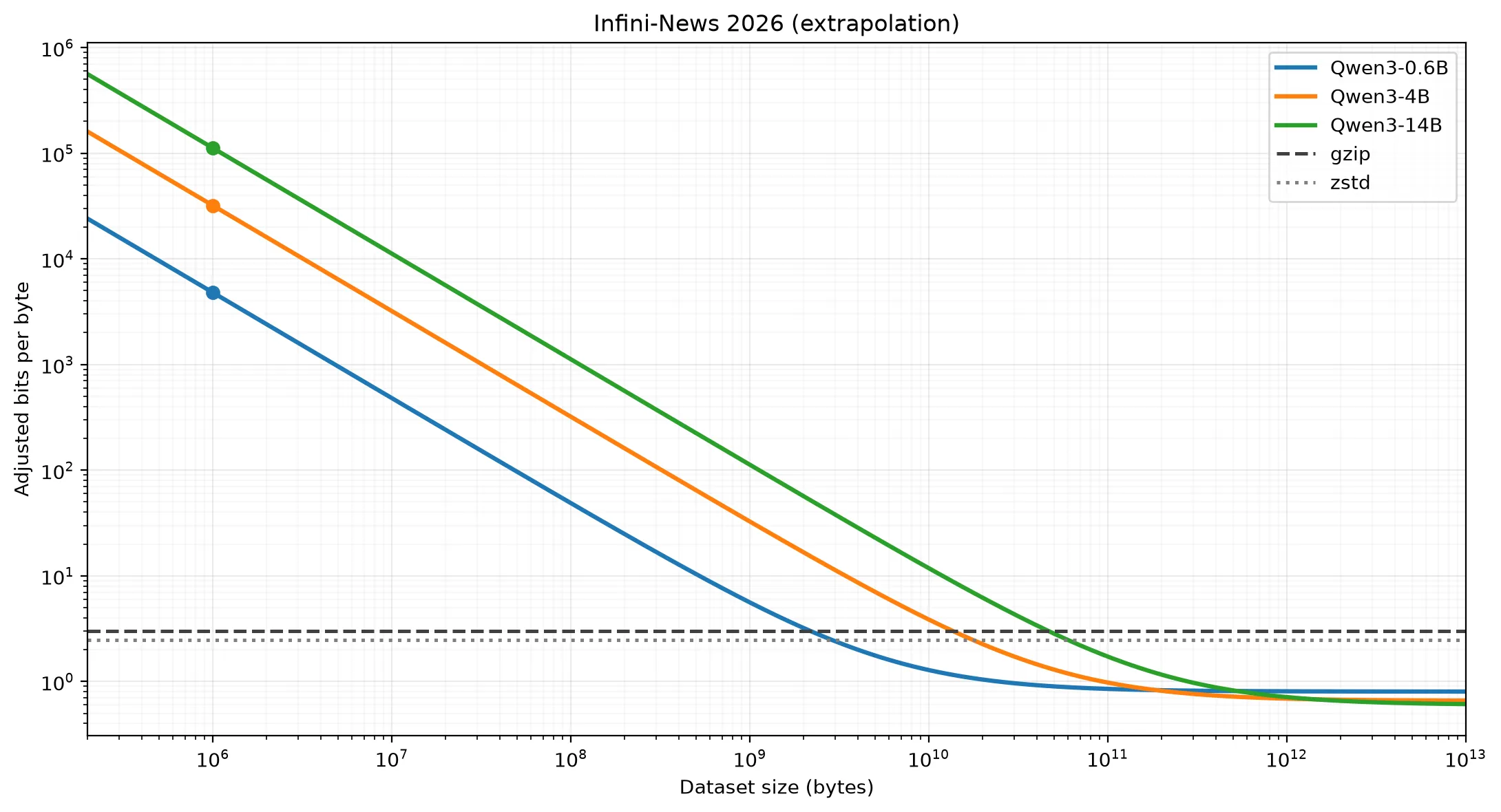
With a sufficiently large dataset — around 2.88 GB for Qwen3-0.6B — the weights become amortized enough to beat zstd in bpb. But is there a way to dispense with the cost of the weights altogether, allowing us to effectively leverage language models as powerful lossless compressors for much smaller datasets, like these?

Online Compression

Consider the geometry of the pretraining loss curve. The x-axis denotes which training step the model is on, and the y-axis the cross-entropy of the data in that step — the mean number of bits needed to encode the data in that batch. The cost of a learner to encode its training dataset is then proportional to the area under the curve, the cumulative sum of the loss across all of the training steps (plus the small constant cost of the code of the learner itself), independent of the size of its weights.

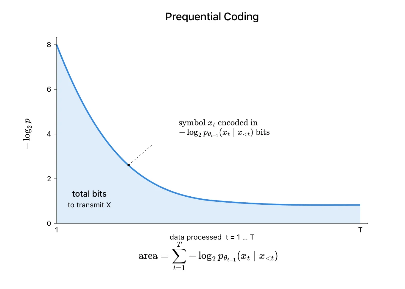
In order for a decoder to be able to retrieve the dataset at each step, the encoder and the decoder must start with the same initial weights. But since we’re learning from scratch, we don’t actually need to transmit the information of the parameters at all, we just need to instantiate them with the same random seed⁴. If we do this, and train the encoder and decoder with the same program deterministically (e.g. with deterministic CUDA kernels), we can transmit the each batch sequentially with the current weights and train the encoder and decoder on them in lockstep, always retaining identical weights on both.

This procedure is called prequential coding (Dawid, 1984; Rissanen, 1984; Blier & Ollivier, 2018). The length of the prequential code is the cumulative sum of all the losses at each step, plus the constant program cost $c$:

To reiterate, the algorithm for prequential coding is as follows:

1. Initialize $\theta_0$ with a fixed random seed on both the encoder and decoder
2. Transmit $x_t$ from the encoder to the decoder in $-\log_2 p_{\theta_{t-1}}\left(x_t \mid x_{\lt t}\right)$ bits
3. Use the $-\log_2 p_{\theta_{t-1}}\left(x_t \mid x_{\lt t}\right)$ bits to decode the original ${x_t}$ on the decoder
4. Do a training step on $x_t$ on both the encoder and decoder, producing $\theta_{t}$
5. Repeat steps 2 through 4 for all $T$

By initializing the weights tabula rasa with the same random seed, and training deterministically on the same data each step, the encoder and decoder share identical weights throughout the entire run without ever transmitting the weights: just the code to randomly initialize them and the data bitstream specified by the training loss curve.

In order to demonstrate this, we will start with an efficient Transformer pretraining codebase borrowed from qlabs-eng/slowrun. The model used has 220M parameters and a simple byte-level tokenizer, and will again be trained deterministically, using the constriction arithmetic coding implementation used to encode the dataset as a bitstream, one $x_t$ at a time. The same hyperparameters are used for all of the datasets.

Doing this on the same three datasets used earlier, we get the following:

Despite the extremely small dataset sizes relative to typical pretraining runs, our model was still able to learn quickly enough to (narrowly) outperform gzip and zstd on all three datasets; most decisively Finnegans Wake, whose diverse and semantically dense vocabulary was significantly harder for the traditional algorithms to compress.

For a larger-scale comparison, we can look to the Large Text Compression Benchmark (Mahoney, 2006): a competition to compress $10^8$ and $10^9$ byte subsets of the English Wikipedia — the compute-unrestricted counterpart of the Hutter Prize (Hutter, 2006). The current leader on the benchmark is nncp (Bellard, 2024), which uses prequential coding with a specialized Transformer model to compress the datasets in an online fashion. With a better-tuned model and significantly more data to learn from, nncp compresses enwik9 into half as many bits-per-byte as zstd:

Instead of the large fixed cost of the weights, the dominating expense in prequential coding comes from the high early cost in transmitting data before the model is able to predict it well. The more efficiently the program (e.g. the model’s architecture and optimizer) learns from each datum, the stronger its compressive capacities. The models used in these experiments are able to learn efficiently enough to outperform traditional compression algorithms on each dataset while making a complete accounting of the cost of both the data bitstream and the program.

Comparing Costs

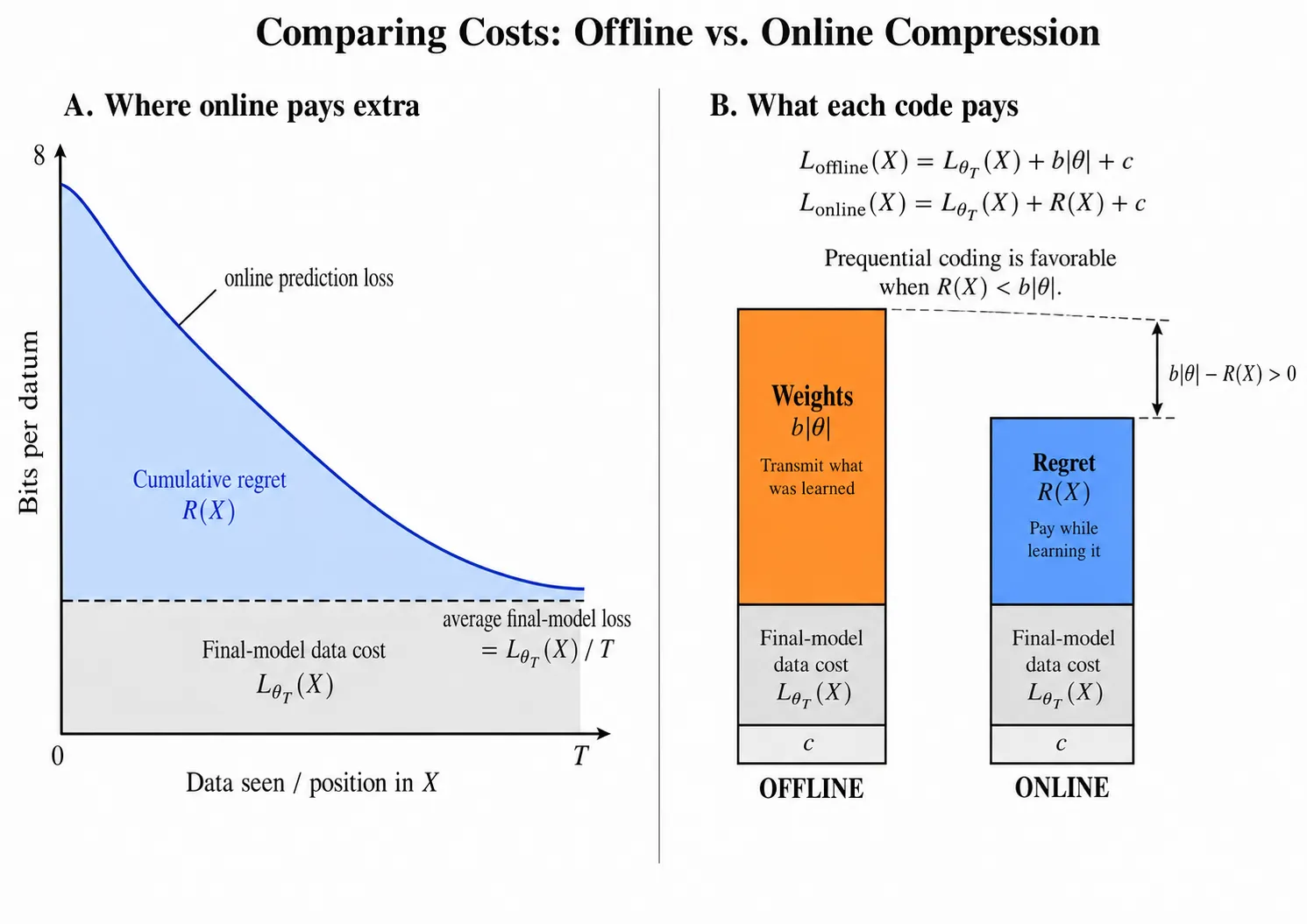
To look more closely at the difference in terms that offline and online charge for compression, consider the final weights of a model $\theta_T$ pretrained on $X$. The cost of encoding $X$ with the final weights $\theta_T$ is:

This is a one-part code of the same form as the first table in the offline section, but we are now using the final weights of a model pretrained on $X$ instead of an externally pretrained model (e.g. Qwen3), so that both the offline and online settings can refer to the same object. Define the learner’s cumulative regret to its own final weights as the excess the online code paid over that bitstream:

Geometrically, $R(X)$ is the area between the learner’s loss curve and its final loss: the bulge of early prediction errors above the floor the model eventually reaches. The two codelengths then decompose as:

With the shared terms cancelling, the comparison reduces to a single asymmetry: offline pays $b|\theta|$, the cost to store the weights; online pays $R(X)$, the cost to learn them. Prequential coding is favorable whenever $R(X) \lt b|\theta|$ — when the structure of $X$ is cheaper to acquire through experience than to transmit the model itself.

Part Two: Intelligence

We have seen that all prediction is implicitly compression, that the pretraining objective explicitly minimizes the description length of $X$, that in the offline setting more powerful pretrained models are able to compress datasets into fewer bits (when either ignoring the cost of their weights or amortizing them with a large enough dataset), and that in the online setting a more efficient learner is able to compress its training dataset into fewer bits.

But what exactly is this property that makes data compressible, and what does it have to do with intelligence?

Generalization

When considering just the data bitstream term, the description length of $X$ is inversely proportional to how well the model $\theta$ predicts it: the more probability $\theta$ places on the true $x_t$, the fewer the bits needed to encode it.

Consider the maximally naive model $u$, which assigns uniform probability to every possible symbol regardless of context: $u\left(x_t \mid x_{\lt t}\right) = 1/|\mathcal{X}|$, where $\mathcal{X}$ is the vocabulary that $X$ is built from. Its codelength is fixed at $L_u(X) = T \log_2 |\mathcal{X}|$ for every $X$. For byte-level data, such as a plaintext UTF-8 dataset, $L_u(X)$ is the raw size of the uncompressed dataset. So long as $-\log_2 p_\theta\left(x_t \mid x_{\lt t}\right)$ is on average smaller than $-\log_2 u\left(x_t \mid x_{\lt t}\right)$, the model $\theta$ encodes the data bitstream in fewer bits than the raw data itself, thereby compressing it: $L_\theta(X) \lt L_u(X)$.

For the complete description length of $X$ — the cost of the data bitstream plus the cost of the program that produced it, as in $L_\text{offline}(X)$ and $L_\text{online}(X)$ — to be smaller than $L_u(X)$, the data bitstream’s savings over the uniform encoding must be greater than the cost of the program.

A program with $X$ hard-coded verbatim can predict it perfectly, making $L_\theta(X) = 0$. But hardcoding a symbol costs at least as many program-bits as it saves in data-bits, so it can never shorten the complete description length; the only bits that turn a profit are those reused across many predictions, where one bit of program pays for itself multiple times in data savings. The extent to which the complete description length is shorter than $L_u(X)$ is therefore the strength of evidence that the program captured reusable predictive structure of $X$.

In offline compression, the pretrained model learned its predictive structure from a training dataset $D$ and reused it to predict the test data $X$; in online compression, $X$ serves as both training and test data, with structure learned from $x_{\lt t}$ reused to predict $x_t$. In both, every profitable bit has the same shape: extracted from prior experience, spent on new data.

This is our operational definition of generalization: the capacity to reuse learnings from prior experience to accurately model novel data.

“Reuse” means the cost of the program is amortized across its predictions, “accurately model” means the cost of the data is small, and the shift from “prior experience” to “novel data” means the accounting is done on data that played no part in building the model. A model generalizes to $X$ along two axes: how far its complete description length falls below $L_u(X)$, and how far $X$ lies from its prior experience.

The Ideal Limits

The cost of describing $X$ with none of its regularities captured was seen to be $L_u(X)$. The theoretical floor of the description length is the Kolmogorov complexity $K(X)$: the length of the shortest program that outputs $X$. $K(X)$ exploits all of the possible reusable structure within $X$, and is bounded by the irreducible noise within the data. It is the ideal limit in an offline setting where all of $X$ is observable up front, but it is unfortunately incomputable, as determining it would require exhaustively evaluating all possible programs, some of which will never halt.

In the online setting, when $X$ instead arrives as a stream, the ideal is Solomonoff induction. Its universal mixture considers every possible program (on a fixed universal monotone machine $U$) whose output begins with $x_{\leq t}$, weighted by an exponential penalty on its length, so that each additional bit of description halves its prior:

We can condition the mixture on the prefix to create a predictor, $M(x_t \mid x_{\lt t})$, and therefore also a prequential code:

It is worth once again emphasizing that each program’s weight is determined solely by its length: its predictions are exponentially concentrated on the continuations favored by the shortest programs. Solomonoff’s theorem proves the mixture is universal: for every computable predictor $q$ and every $X$, $L_M(X) \leq L_q(X) + K(q) + O(1)$, where the right-hand terms specify the cost of $q$‘s two-part code, plus a constant overhead from the choice of universal machine.

The programs that best compress the past dominate the optimal induction’s predictions of the future: a vindication of the relation between compression and generalization. Solomonoff’s theorem lends support to the information-theoretic restatement of Occam’s razor, the Minimum Description Length principle, which states that the shortest complete description of the data is the best model: a pragmatic razor based on the theoretical ideal.

Intelligence

The operational definition of intelligence we will be considering is the capacity to generalize. We will be looking at this capacity in LLMs from two views of the model’s ability to compress novel data, mirroring the two means of compression from Part One.

The offline intelligence view evaluates the final weights of a trained model to measure how well it predicts held-out data. The intelligence of frontier models is evaluated and compared on a variety of real-world benchmarks, such as SWE-bench, FrontierMath, and GDPval, while community training competitions like modded-nanogpt and the slowrun target the final loss of held-out pretraining data — the same quantity measured in Part One. The implicit assumption underlying the faith in these evaluations is that the results are the fruit of generalization: that improved performance isn’t the result of narrow benchmark-maxing, but captures the model’s capacity to broadly generalize to novel data.

The online intelligence view evaluates the rate at which a model learns from experience, commonly referred to as data or sample efficiency. Inside the learning process, data efficiency is the manifestation of generalization: the model is able to better predict $x_t$ if it learned more reusable structure from the data in $x_{\lt t}$ — its capacity to do so approaches the limit of Solomonoff induction.

We will next take a closer look at offline and online intelligence and at their relation with compression.

Offline Intelligence

The offline view of the intelligence of a model looks at how well its frozen final weights predict held-out data. The broader and more diverse the data, the greater the model’s capacity for generalization must be to make accurate predictions. This makes held-out pretraining-like datasets — evaluated by their cross-entropy loss, as done in Part One — among the most robust measures of offline intelligence, as their corpora span an enormous breadth and diversity.

Indeed, the success of the GPT pretraining paradigm was twofold: it demonstrated scaling laws where just by using bigger models and more data you can pretrain better and better compressors, and that those compressive capacities are highly predictive of held-out benchmarks testing what humans deem as intelligent behavior.

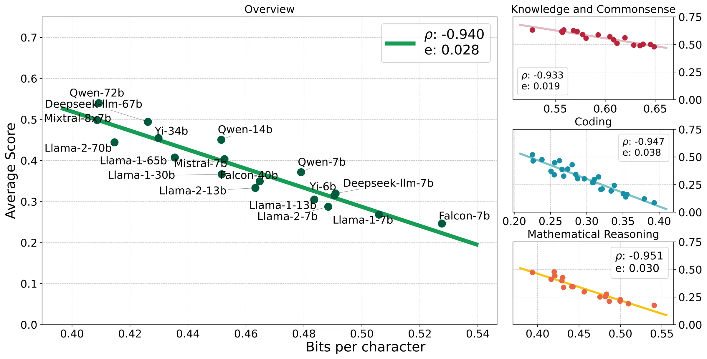
This was elegantly displayed in Compression Represents Intelligence Linearly by Huang et al. (2024). They took thirty-one open-weight pretrained models trained by a variety of labs, and evaluated each model’s compressive capacities on pretraining-like datasets sourced after the models’ knowledge cutoff along with their performance on knowledge and reasoning benchmarks. Plotting the relationship, they found a nearly linear correlation between the two:

However, evaluating a model from its frozen final weights alone — whether by held-out loss or benchmark scores — leaves us unable to account for the training process that produced them. The degree to which a model’s performance demonstrates generalization depends on how far the evaluated data lies from the model’s training distribution, and when evaluating a black-box pretrained model given just its weights, we cannot know what that distance is.

There are strong incentives for even the most well-intentioned labs to include data that, if not the test itself, is the closest data to it that they can justify including. The more the data selection process is skewed towards particular tests, the less representative the final model’s performance on them will be of generalization.

As an illustrative example, in this paper the authors found the Qwen series punched significantly above its compressive weight on the mathematical reasoning benchmarks, “which implies that the Qwen model series may be exposed to the GSM8K training data, MATH training data, and even the MATH test data in the pretraining stage.”⁵

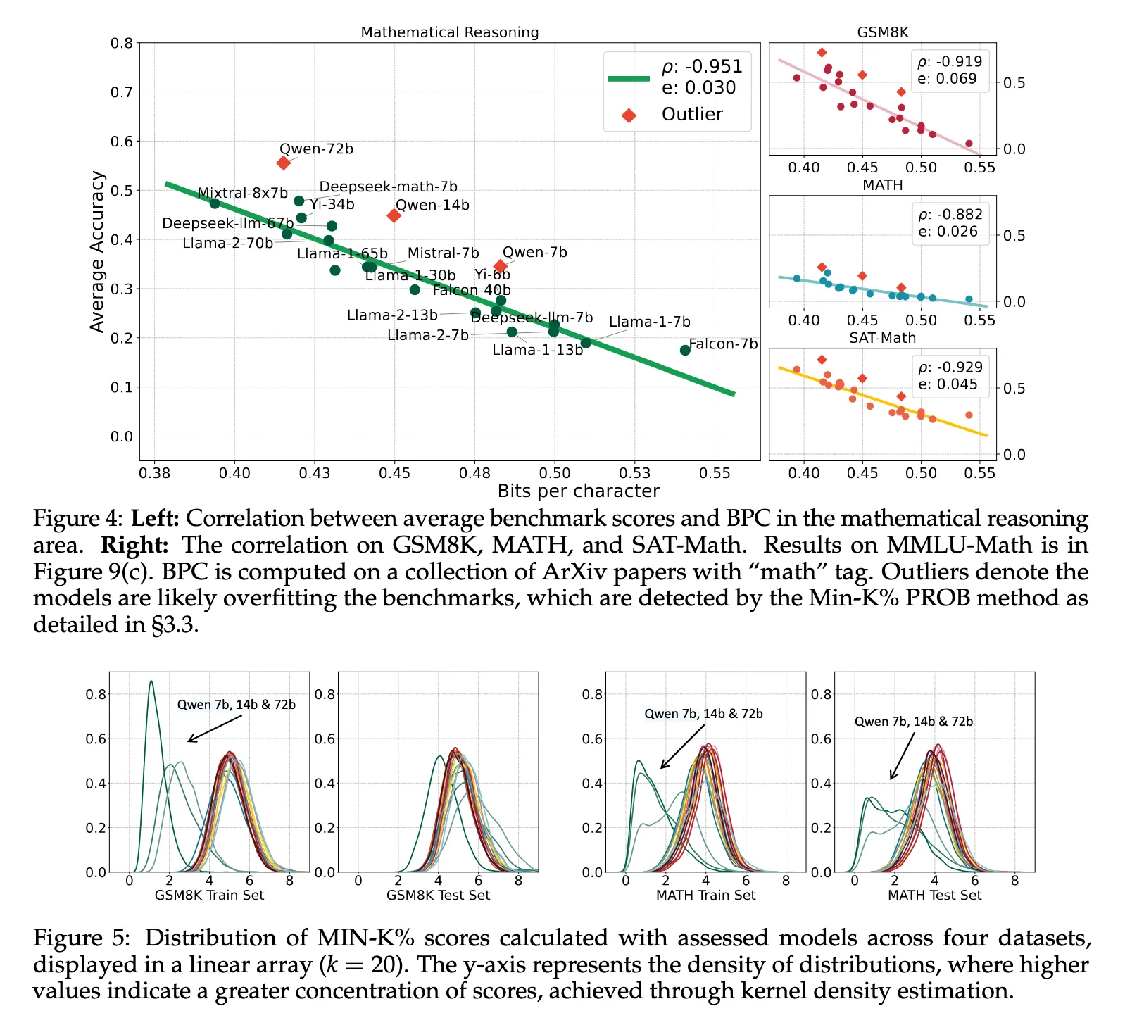
The Huang et al. results thus do double duty: the linear fit supports compression as a measure of the kind of intelligence that the benchmarks target, while the outliers warn against reading too much into benchmark scores themselves — benchmark performance can be easily bought with proximate training data. In their experiments, loss on broad pretraining corpora proved harder to game, but in measurements of offline intelligence we can never in principle be sure how skewed training was to those corpora either.

The deepest problem with offline measures of intelligence is that evaluations of the final artifact of training cannot account for the process that produced it, and therefore cannot account for the degree to which its performance is the result of generalization. To evaluate the process of learning itself, we now turn to online intelligence.

Online Intelligence

The online view of intelligence asks how efficiently the learner turns experience into generalization. In this view, no measure of the final artifact of training alone can be a measure of intelligence, because intelligence is fundamentally a property of the learner.

This is the same distinction made in Chollet (2019) between skill and skill-acquisition, in which “skill” refers to a system’s performance on task-specific tests (e.g. real-world benchmarks or loss on pretraining corpora), while “skill-acquisition” refers to a system’s ability to learn new tasks. Chollet argues that

solely measuring skill at any given task falls short of measuring intelligence, because skill is heavily modulated by prior knowledge and experience: unlimited priors or unlimited training data allow experimenters to “buy” arbitrary levels of skills for a system, in a way that masks the system’s own generalization power.

To tie this back to compression, an offline measure of intelligence can charge a cost for the program $b|\theta| + c$ (though it rarely does — as in Huang et al.’s exclusion of the cost of the weights), but the program cost makes the contributions of prior knowledge and experience invisible. When making offline comparisons of models of the same architecture, one that was warm-started from a previous run, one that was trained on one billion tokens, and one that was trained on a trillion tokens will have identical program costs despite vastly differing amounts of prior knowledge and experience.

If you recall from Part One, prequential coding dispenses with the cost of the weights, charging instead the cost of experience to train the model tabula rasa:

The formulation of prequential coding enables us to charge and quantify the prior⁶ and experience of a learner in a unified measure, the prequential codelength. Where Part One looked at $L_{\text{online}}(X)$ purely from the perspective of compression, we will now view it as a measure of data efficiency — a measure of online intelligence.

Define a learner’s data efficiency on $X$ as the average number of bits of predictive value it extracts per datum of experience. Since the prequential codelength is the learner’s total prediction cost over $X$, a shorter codelength on the same $X$ is greater data efficiency: the learner paid fewer bits for the same experience. And to pay fewer bits for $x_t$ is to have better generalized from $x_{\lt t}$ — to have converted prior experience into more structure reusable for predicting novel data. The prequential codelength thus unifies generalization, data efficiency, and the learner’s complete description length of $X$ into a single quantity.

When comparing learners by $L_{\text{online}}(X)$, one confounder remains uncharged: the data-dependent difficulty in generalizing to $x_t$ from $x_{\lt t}$. Different experiences $X$ have different inherent amounts of reusable structure and difficulties of learning that structure. There are no known practical methods to quantify this dataset-dependent difficulty, so we can’t charge for it, and must instead control for it by comparing learners trained on the same distribution of data, in the same order.

Consider a comparison of two learners trained on the same $X$, where Learner A is more efficient across the board, dominating Learner B at every point on the loss curve. If we were to compare Learner A halfway through its training to Learner B trained on the entire dataset, they would be indistinguishable in terms of offline intelligence as measured by pretraining loss.

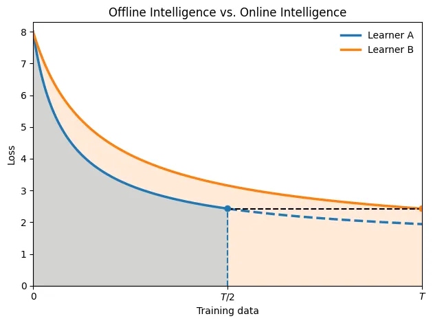
In contrast, when evaluated in terms of online intelligence — their prequential codelength, as depicted by the shaded area under the curve — Learner A is significantly more intelligent than Learner B, which had a higher cost per datum at every point in the curve, and therefore also needed more data to reach the same loss.

However, neither of the scalars — offline loss nor prequential codelength — is scale-invariant. Both evaluations occur at a specific amount of experience $T$, and the verdict can flip as $T$ grows.

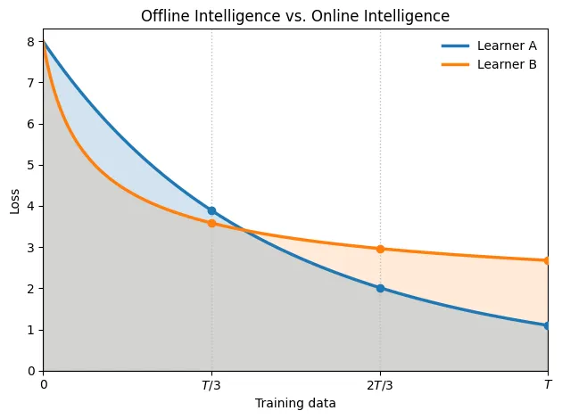
At $T/3$, Learner B has both a lower loss and a shorter prequential code than Learner A; at $2T/3$, Learner B has a higher loss but still the shorter code; by $T$, Learner A has overtaken Learner B on both metrics.

To get a scale-invariant comparison of learners, we must turn from particular training loss curves to their underlying geometry: the rules that govern their loss at arbitrary levels of experience.

Intelligence at Scale

Empirically, the training loss curves of pretraining can be closely modeled by power laws. By fitting a few coefficients that capture different properties of the learner we can predict its loss at an arbitrary $t$:

The coefficients form the geometry of the loss curve. $H$ is the floor the learner converges toward: bounded below by the intrinsic entropy of the data, and above by the representational capacity of the model. The excess loss above the floor, $B\,t^{-\beta}$, is a power law — on log-log axes a straight line, with slope $-\beta$ and $B$ its level. $\beta$ tilts the curve; $B$ shifts it wholesale, a constant multiplicative factor at every $t$, and all three play a role in determining the learner’s data efficiency.

Prequential codelength inherits this geometry analytically. Summing the loss over the entirety of $T$, with the addition of the cost of the program $c$, and evaluating the sum — for $\beta < 1$, the regime empirical exponents occupy — the codelength splits into three terms of strictly decreasing order of growth:

In the loss curve, $B\,t^{-\beta}$ decays to zero: every learner converges to its floor. Each coefficient thus governs a term of a different order in the prequential codelength: $H$ the linear term of the floor, $1 - \beta$ which determines the exponent of the sublinear term (which is the learner’s regret to $H$⁷), $B$ its prefactor, and $c$ the constant cost of the program. The ordering of the coefficients follows from the ordering of their terms: as $T$ grows, any difference in a higher-order term eventually swamps any difference in a lower-order one.

Therefore, in the limit — as $T \to \infty$ — the only term that matters is $H$. But in practice, $T$ is bounded: the pretraining datasets used by frontier labs are approaching all available high-quality data on the Internet (Villalobos et al., 2024).

Patel (2026) estimates that humans acquire language and learn to drive from three to six orders of magnitude less experience than models: an existence proof of how much room in data efficiency remains. Where before we could compensate for learning less from each token by training on many more tokens, today the limit is set by the data efficiency of the learner.

Related Works

The identity between prediction and compression begins with Shannon (1948). Arithmetic coding (Pasco, 1976; Rissanen, 1976; Witten, Neal & Cleary, 1987) converts any predictor’s probabilities into a bitstream at negligible overhead.

The ideal limits belong to algorithmic information theory. Solomonoff (1964) defined the universal mixture and later proved its convergence (Solomonoff, 1978); Kolmogorov (1965) and Chaitin (1966) independently formalized descriptive complexity.

The insistence that a complete description must charge for the program predates its name: Wallace & Boulton (1968) proposed two-part codes as Minimum Message Length a decade before Rissanen (1978) founded Minimum Description Length. Hinton & van Camp (1993) brought the charge for the weights to neural networks. The online alternative, prequential coding, was developed by Dawid (1984) and Rissanen (1984); Blier & Ollivier (2018) showed that prequential codes of deep networks are dramatically shorter than their two-part counterparts, and Jiang & Zhou (2025) give an excellent intuitive treatment applied to data curricula. Concurrent work from Qiu (2026) proposes requential coding as a means to produce shorter descriptions than prequential coding, at the cost of being even more computationally expensive.

In practice, Delétang et al. (2023) demonstrated pretrained LLMs as offline compressors, while Mahoney’s Large Text Compression Benchmark (2006) and its current leader nncp (Bellard, 2024) represent the state of the art of prequential coding on the enwik8 and enwik9 datasets.

Chaitin has long held that comprehension is compression (Chaitin, 2002). Hutter (2005) extended Solomonoff induction to optimal agency with AIXI, and Legg & Hutter (2007) built a formal definition of universal intelligence atop it. Text compression was proposed as a test by Mahoney (1999), and formalized by the Hutter Prize (Hutter, 2006). This thesis is strong within certain groups at frontier labs: publicly, Rae (2023) argued for compression as the path to AGI, Sutskever (2023) framed SGD as a compressor to explain unsupervised learning, and Selsam (2025) described pretraining as approximate Solomonoff induction. Huang et al. (2024) measured the relation between compression and benchmark performance and found it linear. Chollet (2019)‘s decoupling of intelligence into separate skill and skill-acquisition camps was motivation for the essay’s mapping between offline and online intelligence.

The power laws used to model training loss curves come from the scaling law literature (Hestness et al., 2017; Kaplan et al., 2020; Hoffmann et al., 2022), and Villalobos et al. (2024) documents the approaching data wall. The slowrun (qlabs et al., 2025) is an exemplar public competition in data efficient training algorithms.

Finally, to avoid being Schmidhuber’d, yes, he has long argued for a relation between compression and intelligence, and Schmidhuber (2009) in particular sits among my favorite papers.

Conclusion

Every predictor is a compressor, and an honest accounting of compression must include the cost of the program. The only way for the complete description length of data to be shorter than the raw data itself is through capturing reusable structure whose cost in program bits is less than the bits it saves in accurately modeling the data, and to do this on data never previously seen is to generalize.

Intelligence is the capacity to generalize. We examined it from two views: offline, evaluating the compressive capacities of pretrained models on held-out datasets, where it has a nearly linear relation with benchmarks of intelligent behavior, and online, evaluating the learner itself, where generalization was identified with data efficiency. In both, intelligence was measured in bits.

As frontier pretraining runs approach the wall of all high-quality data on the internet, increased intelligence must come from closing the data efficiency gap between models and humans. The more efficient the learner, the shorter its complete description length of the dataset, and the closer it approximates the ideal of Solomonoff induction.

Acknowledgements

Thank you to Niloofar Mireshghallah, Samip Dahal, Liam Corrigan, and Fable 5 for early comments on the draft, and Lambda for sponsoring the compute used for the experiments of Part One.

Citation

@article{greene2026intelligence,
  title = {Compression and Intelligence},
  author = {Greene, Ryan},
  journal = {greene.sh},
  year = {2026},
  month = {July},
  url = "https://www.greene.sh/compression-and-intelligence/"
}

References

• Fabrice Bellard. “NNCP: Lossless Data Compression with Neural Networks.”. Technical report, bellard.org (2024).
• Léonard Blier and Yann Ollivier. “The Description Length of Deep Learning Models.”. Advances in Neural Information Processing Systems 31 (2018).
• Gregory J. Chaitin. “On the Length of Programs for Computing Finite Binary Sequences.”. Journal of the ACM 13 (4): 547–569 (1966).
• Gregory J. Chaitin. “On the Intelligibility of the Universe and the Notions of Simplicity, Complexity and Irreducibility.” Lecture, German Philosophy Congress, Bonn (2002).
• François Chollet. “On the Measure of Intelligence.”. arXiv preprint arXiv:1911.01547 (2019).
• A. Philip Dawid. “Present Position and Potential Developments: Some Personal Views: Statistical Theory: The Prequential Approach.”. Journal of the Royal Statistical Society, Series A 147 (2): 278–292 (1984).
• Grégoire Delétang, Anian Ruoss, Paul-Ambroise Duquenne, Elliot Catt, Tim Genewein, et al. “Language Modeling Is Compression.”. International Conference on Learning Representations (2023).
• Joel Hestness, Sharan Narang, Newsha Ardalani, Gregory Diamos, Heewoo Jun, et al. “Deep Learning Scaling Is Predictable, Empirically.”. arXiv preprint arXiv:1712.00409 (2017).
• Geoffrey E. Hinton and Drew van Camp. “Keeping the Neural Networks Simple by Minimizing the Description Length of the Weights.”. Proceedings of the Sixth Annual Conference on Computational Learning Theory: 5–13 (1993).
• Jordan Hoffmann, Sebastian Borgeaud, Arthur Mensch, Elena Buchatskaya, Trevor Cai, et al. “Training Compute-Optimal Large Language Models.”. Advances in Neural Information Processing Systems 35 (2022).
• Yuzhen Huang, Jinghan Zhang, Zifei Shan, and Junxian He. “Compression Represents Intelligence Linearly.”. Conference on Language Modeling (2024).
• Marcus Hutter. Universal Artificial Intelligence: Sequential Decisions Based on Algorithmic Probability. Springer (2005).
• Marcus Hutter. “The Hutter Prize for Lossless Compression of Human Knowledge.”. prize.hutter1.net (2006).
• Yiding Jiang and Allan Zhou. “A Compression Perspective on Curriculum Learning.”. Blog post, yidingjiang.github.io (2025).
• Jared Kaplan, Sam McCandlish, Tom Henighan, Tom B. Brown, Benjamin Chess, et al. “Scaling Laws for Neural Language Models.”. arXiv preprint arXiv:2001.08361 (2020).
• Andrey N. Kolmogorov. “Three Approaches to the Quantitative Definition of Information.” Problems of Information Transmission 1 (1): 1–7 (1965).
• Ruggero Marino Lazzaroni, Jana Lasser, and Kirill Solovev. “Infini-News: Efficiently Queryable Access to 1.3 Billion Processed Common Crawl News Articles.”. arXiv preprint arXiv:2605.18337 (2026).
• Shane Legg and Marcus Hutter. “Universal Intelligence: A Definition of Machine Intelligence.”. Minds and Machines 17 (4): 391–444 (2007).
• Matthew V. Mahoney. “Text Compression as a Test for Artificial Intelligence.” Proceedings of AAAI-99 (1999).
• Matthew V. Mahoney. “Large Text Compression Benchmark.”. mattmahoney.net (2006).
• Richard C. Pasco. “Source Coding Algorithms for Fast Data Compression.” Ph.D. thesis, Stanford University (1976).
• Dwarkesh Patel, “The data black hole at the center of AI”, Dwarkesh Podcast, June 19, 2026.
• Shikai Qiu, Marc Finzi, Yujia Zheng, Kun Zhang, and Andrew Gordon Wilson. “Requential Coding: Pushing the Limits of Model Compression with Self-Generated Training Data.”. arXiv preprint arXiv:2607.11883 (2026).
• qlabs. “slowrun.”. GitHub repository (2025).
• Jack Rae. “Compression for AGI.”. Stanford MLSys Seminar #76 (2023).
• Jorma Rissanen. “Generalized Kraft Inequality and Arithmetic Coding.”. IBM Journal of Research and Development 20 (3): 198–203 (1976).
• Jorma Rissanen. “Modeling by Shortest Data Description.”. Automatica 14 (5): 465–471 (1978).
• Jorma Rissanen. “Universal Coding, Information, Prediction, and Estimation.”. IEEE Transactions on Information Theory 30 (4): 629–636 (1984).
• Jürgen Schmidhuber. “Driven by Compression Progress: A Simple Principle Explains Essential Aspects of Subjective Beauty, Novelty, Surprise, Interestingness, Attention, Curiosity, Creativity, Art, Science, Music, Jokes.”. arXiv preprint arXiv:0812.4360 (2009).
• Daniel Selsam. “Pre-Training GPT-4.5.”. OpenAI podcast with Sam Altman, Alex Paino, and Amin Tootoonchian (2025).
• Claude E. Shannon. “A Mathematical Theory of Communication.”. Bell System Technical Journal 27 (3): 379–423 and 27 (4): 623–656 (1948).
• Ray J. Solomonoff. “A Formal Theory of Inductive Inference. Parts I and II.”. Information and Control 7 (1): 1–22 and 7 (2): 224–254 (1964).
• Ray J. Solomonoff. “Complexity-Based Induction Systems: Comparisons and Convergence Theorems.”. IEEE Transactions on Information Theory 24 (4): 422–432 (1978).
• Ilya Sutskever. “An Observation on Generalization.”. Simons Institute Workshop on Large Language Models and Transformers, UC Berkeley (2023).
• Pablo Villalobos, Anson Ho, Jaime Sevilla, Tamay Besiroglu, Lennart Heim, and Marius Hobbhahn. “Will We Run Out of Data? Limits of LLM Scaling Based on Human-Generated Data.”. Proceedings of the 41st International Conference on Machine Learning (2024).
• Christopher S. Wallace and David M. Boulton. “An Information Measure for Classification.”. The Computer Journal 11 (2): 185–194 (1968).
• Ian H. Witten, Radford M. Neal, and John G. Cleary. “Arithmetic Coding for Data Compression.”. Communications of the ACM 30 (6): 520–540 (1987).
• An Yang, Anfeng Li, Baosong Yang, Beichen Zhang, Binyuan Hui, et al. “Qwen3 Technical Report.”. arXiv preprint arXiv:2505.09388 (2025).

Footnotes